Examples

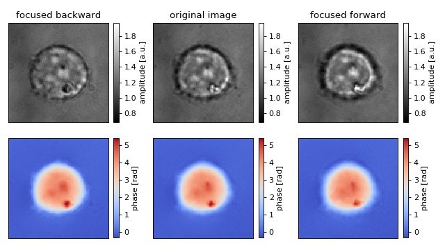
2D Refocusing of an HL60 cell

The data show a live HL60 cell imaged with quadriwave lateral shearing interferometry (SID4Bio, Phasics S.A., France). The diameter of the cell is about 20µm.

refocus_cell.py

import matplotlib.pylab as plt
from skimage.restoration import unwrap_phase
import numpy as np

import nrefocus

from example_helper import load_cell

# load initial cell
cell1 = load_cell("HL60_field.zip")

# refocus to two different positions
cell2 = nrefocus.refocus(cell1, 15, 1, 1)  # forward
cell3 = nrefocus.refocus(cell1, -15, 1, 1)  # backward

# amplitude range
vmina = np.min(np.abs(cell1))
vmaxa = np.max(np.abs(cell1))
ampkw = {"cmap": plt.get_cmap("gray"),
         "vmin": vmina,
         "vmax": vmaxa}

# phase range
cell1p = unwrap_phase(np.angle(cell1))
cell2p = unwrap_phase(np.angle(cell2))
cell3p = unwrap_phase(np.angle(cell3))
vminp = np.min(cell1p)
vmaxp = np.max(cell1p)
phakw = {"cmap": plt.get_cmap("coolwarm"),
         "vmin": vminp,
         "vmax": vmaxp}

# plots
fig, axes = plt.subplots(2, 3, figsize=(8, 4.5))
axes = axes.flatten()
for ax in axes:
    ax.xaxis.set_major_locator(plt.NullLocator())
    ax.yaxis.set_major_locator(plt.NullLocator())

# titles
axes[0].set_title("focused backward")
axes[1].set_title("original image")
axes[2].set_title("focused forward")

# data
mapamp = axes[0].imshow(np.abs(cell3), **ampkw)
axes[1].imshow(np.abs(cell1), **ampkw)
axes[2].imshow(np.abs(cell2), **ampkw)
mappha = axes[3].imshow(cell3p, **phakw)
axes[4].imshow(cell1p, **phakw)
axes[5].imshow(cell2p, **phakw)

# colobars
cbkwargs = {"fraction": 0.045}
plt.colorbar(mapamp, ax=axes[0], label="amplitude [a.u.]", **cbkwargs)
plt.colorbar(mapamp, ax=axes[1], label="amplitude [a.u.]", **cbkwargs)
plt.colorbar(mapamp, ax=axes[2], label="amplitude [a.u.]", **cbkwargs)
plt.colorbar(mappha, ax=axes[3], label="phase [rad]", **cbkwargs)
plt.colorbar(mappha, ax=axes[4], label="phase [rad]", **cbkwargs)
plt.colorbar(mappha, ax=axes[5], label="phase [rad]", **cbkwargs)

plt.suptitle("Refocused cell on CPU with Numpy")
plt.tight_layout()
plt.show()

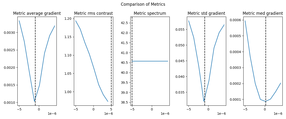
Compare available Metrics for Refocusing

The HL60 cell data used is described in refocus_cell.py.

compare_metrics.py

import nrefocus
from nrefocus.metrics import METRICS
import matplotlib.pyplot as plt

from examples.example_helper import load_cell

nrefocus.set_ndarray_backend("cupy")

dataset = load_cell("HL60_field.zip")

# load initial cell and create rf object
rf = nrefocus.iface.RefocusCupy(field=dataset,
                                wavelength=647e-9,
                                pixel_size=0.139e-6,
                                kernel="helmholtz")

# autofocus the image for each metric
my_metrics = list(METRICS.keys())

fig, axes = plt.subplots(1, len(my_metrics), figsize=(12, 5))

for i, mt in enumerate(my_metrics):
    af_vals = rf.autofocus(metric=mt,
                           minimizer="legacy",
                           interval=(-5e-6, 5e-6),
                           ret_field=True,
                           ret_grid=True)
    d, grid, field = af_vals
    d = d.get()
    field = field.get()
    grid_0 = grid[0].get()
    grid_1 = grid[1].get()

    axes[i].plot(grid_0, grid_1)
    axes[i].axvline(d, color='k', ls='--')
    axes[i].set_title(f"Metric {mt}")

fig.suptitle("Comparison of Metrics")
fig.tight_layout()
plt.show()

Refocus a stack of 2D fields (3D array input).

This example shows how to refocus a stack shaped (n, y, x). nrefocus interprets the last two axes as spatial axes and broadcasts over any leading “batch” axes.

refocus_stack.py

import numpy as np

import nrefocus

rng = np.random.default_rng(0)

# Synthetic complex field stack: (n, y, x)
n, ny, nx = 5, 128, 96
amp = 1 + 0.1 * rng.normal(size=(n, ny, nx))
pha = 0.3 * rng.normal(size=(n, ny, nx))
field = amp * np.exp(1j * pha)

pixel_size = 1e-6
dist = 2.13 * pixel_size

# CPU (NumPy) refocus of the entire stack in one call
rf = nrefocus.RefocusNumpy(
    field=field,
    wavelength=8.25 * pixel_size,
    pixel_size=pixel_size,
    medium_index=1.533,
    distance=0,
    kernel="helmholtz",
    padding=True,
)
refocused = rf.propagate(distance=dist)
print("nrefocus now accepts stacks of 2D arrays (3D input)!\n"
      "Input shape:", field.shape, "| Output shape-> ", refocused.shape)

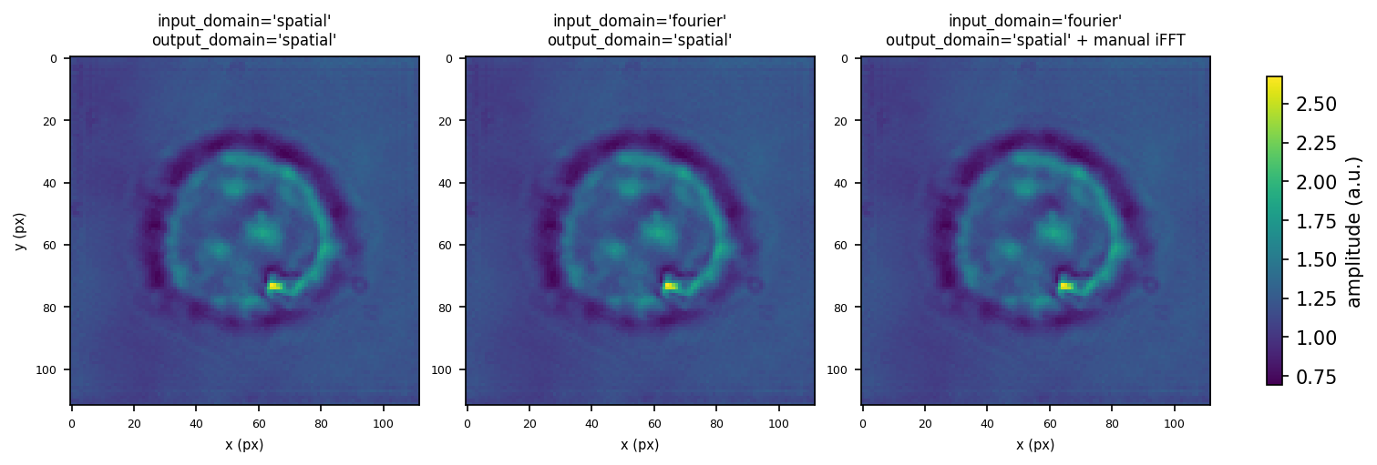
Specifying input_domain / output_domain in nrefocus.

As of version 0.6.2, users can specify in which domain the input and output data exists. The options are ‘spatial’ (default behaviour) and ‘fourier’. These can be used in conjunction with qpretrieve’s ‘output_domain’ to reduce the number of Fourier transforms in a given pipeline (see https://qpretrieve.readthedocs.io/).

Each of the three subplots below produce the same spatial result when padding=False. Note that qpretrieve is not used in this example.

input_output_domains.py

import matplotlib.pyplot as plt
import numpy as np
import nrefocus

from example_helper import load_cell

field = load_cell("HL60_field.zip")
fft_field = np.fft.fftshift(np.fft.fft2(field))

propagation_kwargs = dict(d=15, nm=1, res=1, method="helmholtz", padding=False)

# 1. default (spatial in, spatial out)
refocused_spatial = nrefocus.refocus(field=field, **propagation_kwargs)

# 2. fourier input (skip forward FFT)
refocused_fourier_in = nrefocus.refocus(
    field=fft_field,
    input_domain="fourier",
    **propagation_kwargs,
)

# 3. fourier output, then manual iFFT
refocused_fft_out = nrefocus.refocus(
    field=field,
    output_domain="fourier",
    **propagation_kwargs,
)
# if the field came from qpretrieve, we could use the new feature
# `oah.compute_field(refocused_fft_out)`
refocused_from_fft_out = np.fft.ifft2(np.fft.ifftshift(refocused_fft_out))

assert np.allclose(refocused_spatial, refocused_fourier_in, atol=1e-12), (
    "1 and 2 differ.")
assert np.allclose(refocused_spatial, refocused_from_fft_out, atol=1e-12), (
    "1 and 3 differ after iFFT.")
print("All outputs match:", True)

# plot the output fields
amp = [
    np.abs(refocused_spatial),
    np.abs(refocused_fourier_in),
    np.abs(refocused_from_fft_out),
]
titles = [
    "input_domain='spatial'\noutput_domain='spatial'",
    "input_domain='fourier'\noutput_domain='spatial'",
    "input_domain='fourier'\noutput_domain='spatial' + manual iFFT",
]

vmin = min(a.min() for a in amp)
vmax = max(a.max() for a in amp)

fig, axes = plt.subplots(1, 3, figsize=(10, 3.2), constrained_layout=True)
for ax, a, title in zip(axes, amp, titles):
    im = ax.imshow(a, cmap="viridis", vmin=vmin, vmax=vmax)
    ax.set_title(title, fontsize=8)
    ax.set_xlabel("x (px)", fontsize=7)
    ax.tick_params(labelsize=6)
axes[0].set_ylabel("y (px)", fontsize=7)

fig.colorbar(im, ax=axes, label="amplitude (a.u.)", shrink=0.8)
plt.savefig("input_output_domains.png", dpi=150, bbox_inches="tight")
plt.show()